Visualizing commutative structure in groups
Introducing the commutativity plot to explain basic concepts related to commutativity
Introduction
I built a simple visualization tool, the commutativity plot, that I used to better understand commutativity in finite groups as I was learning about group theory this semester. By the end of this post, I aim to summarize a couple of concepts leading up to two theorems illustrated with this visualization. Namely, we’ll touch on group action, orbits and stabilizers of an element, the permutation representation of groups, conjugation, conjugacy classes, centralizers, and we’ll derive the formula for the number of conjugacy classes. We will also look at why the probability that two randomly picked elements commute in a finite group is a maximum of 5/8 in non-abelian groups, which I find fascinating.
Disclaimer: the function implementation and Mathematica syntax used is very naive, and blows up with larger groups. I am open to PRs, contributions, suggestions for improvements!
Groups acting on sets
One of the most important things you can do with a group is to have it act on a set. The group action has to be valid operations on the set. For example, if the set is the group itself, the action can be left/right multiplication or conjugation (defined later) as well. When we’re talking about an action of an element of the group on a set element in abstract, i.e. without specifying exactly what we mean, we denote it by .
If we apply a group action defined by all elements of on an element , we get a set: , the orbit of . The elements in that keep the same are called the stabilizer of in , denoted . The stabilizer of any element is a subgroup of . In fact the orbit of is an equivalence class for , and the group action divides into disjoint equivalence classes. It is also provable that the order of (the number of elements in) the orbit equals to the index of the stabilizer .
Permutation representation
By Cayley’s theorem, every group of order is isomorphic to some subgroup of , the symmetric group of order . We are going to assume that for the group in question you can generate the permutation representation, specifically the permutation cycle notation of the elements. For example, for the quaternion group , we can list the elements of the group itself using the Quaternions package:
<<Quaternions`
(* Code to generate a group based on its generators and composition
rule, this is brute force, can easily blow up if your generators are
not closed under multiplication, or are too big *)

GenerateGroupElements[generators_, compose_] :=
  FixedPoint[Union[#, compose @@@ Tuples[#, 2]] &, generators];

(* Q8 group = <i,j,k>, composition: quaternion product *)

quaternionGroupElements = GenerateGroupElements[

   {Quaternion[0, 1, 0, 0],  (* i *)
   Quaternion[0, 0, 1, 0],   (* j *)
    Quaternion[0, 0, 0, 1]}, (* k *)
   (#1 ** #2) & (* quaternion product *)
   ];


(* A nice example of Cayley's theorem, where we are acting on G by itself with
left multiplication *)

quaternionGroupPermutations = (el = #;
     FindPermutation[
      quaternionGroupElements, (el ** #) & /@
       quaternionGroupElements]
     ) &  /@ quaternionGroupElements;

(* storing the result in a PermutationGroup object *)
QuaternionGroup = PermutationGroup[quaternionGroupPermutations ]
The above results in:
PermutationGroup[{Cycles[{}],
  Cycles[{{1, 2}, {3, 4}, {5, 6}, {7, 8}}],
  Cycles[{{1, 4, 2, 3}, {5, 8, 6, 7}}],
  Cycles[{{1, 3, 2, 4}, {5, 7, 6, 8}}],
  Cycles[{{1, 6, 2, 5}, {3, 7, 4, 8}}],
  Cycles[{{1, 5, 2, 6}, {3, 8, 4, 7}}],
  Cycles[{{1, 8, 2, 7}, {3, 6, 4, 5}}],
  Cycles[{{1, 7, 2, 8}, {3, 5, 4, 6}}]}]
The permutation representation for groups is akin to the matrix representation of operators on a vector space in a given basis. We can see in this chosen labeling that keeps the elements in place, is a quadruple of transpositions (swaps), and permutes into .
One thing we get with this representation is stable, deterministic ordering between permutations, which will allow for seeing subgroup structure clearly in larger groups.
Conjugacy classes
Fun things happen when a group acts on itself! Two elements, commute when . This is the same as saying , i.e. that is fixed by conjugation by .
If we have act on itself by conjugation, the orbit of an element , a.k.a the disjoint equivalence class, is called the conjugacy class of . The stabilizer subgroup under conjugation for is the subgroup that fixes by conjugation. What does that mean? It means that it’s all the elements commutes with. There is a special name for that: the centralizer of in , denoted . The elements that commute with everything are called the center of , - it is easy to see that the center is the intersection of all the centralizers and hence it is also a subgroup.
It is easy to prove (p 125 in (Dummit & Foote, 2003)) that conjugation preserves the length of the cycles of a permutation, i.e. all the conjugates within a conjugacy class have the same cycle lengths. In Mathematica, you could write a function called CycleLengths that does this calculation.
In[1]:= CycleLengths[c_]:=Sort[Length/@c[[1]]];
CycleLengths[Cycles[{{1,2},{3,4},{5,6},{7,8}}]]
CycleLengths[Cycles[{{1,2},{3,4,5}}]]
Out[2]= {2,2,2,2}
Out[3]= {2,3}
However, even though elements in the same conjugacy class have the same cycle lengths, it doesn’t necessarily work the other direction. To see this there are two examples in mind: abelian groups and the quaternion group.
As everything commutes with everything in abelian groups, the conjugacy class for each element is going to contain only that element. But in a cyclic group of prime order for example all non-trivial elements are of order , their permutation representation looks like . How is that possible? Well, there are no other elements to conjugate them into each other…or to put it another way all elements fix each other by conjugation.
In the quaternion group , have the same cycle lengths but you can only get as far as an element and its inverse in the conjugacy classes. There are no elements in the group that can do the conjugation.
To summarize - conjugacy classes split up into disjoint sets, and while cycle lengths are the same within a conjugacy class, the property of being in a conjugacy class is inherently connected to the group you are in.
The commutativity plot: commuting visibly
To visualize all the ideas above, I coded up a function called CommutativityPlot in this gist. If we order the elements of the group by their conjugacy class and then their natural sorting order (defined by Mathematica), and we plot whether they commute or not, we’ll get a graph plot like this for our quaternion group, :
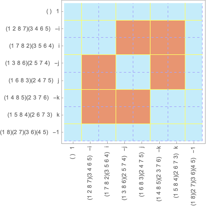
Let’s dissect this!
Each row and column contains the elements that are either commute (blue) or don’t commute (red) with the given element corresponding to that row. The blue squares in a row (or column) are the centralizer for each . If the full row (column) is blue, that means that the element is in the center, .
We know that every element commutes with:
- itself the diagonal is always going to be blue
- the identity the first row and column will always be blue
In the case of , some of the elements are not self-inverse, e.g. , and we know that the elements commute with their inverse. In the current labeling, the inverses are next to each other, that’s why we see the 2x2 blue squares on the diagonal.
Also, notice the yellow grid. As we organized the elements by conjugacy class, a conjugacy class will be a contiguous interval of rows and columns. The intersection of these regions is where the inter-class commutation relations are visible. We can see intra-class commutativity relations outside of the block diagonal squares.
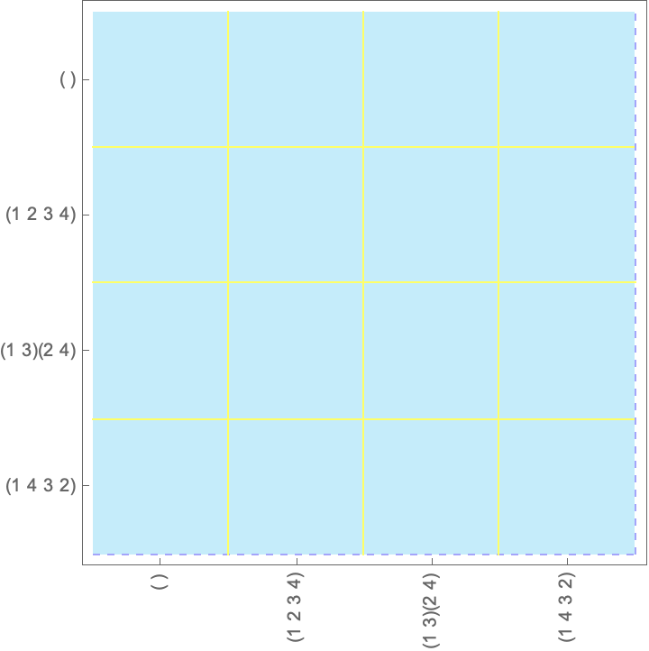
As I mentioned in the previous part, cyclic groups are abelian, every element commutes with each other, thus in the commutativity plot we will have
- a fully blue plot
- conjugacy classes of size 1.
As an example see below the (pretty boring) commutativity plot for the group.
Number of conjugacy classes
Within a conjugacy class (i.e. between two yellow lines), the number of blue squares is going to be the number of elements in the group! Why?
To see this, let’s line up our concepts next to each other in the different “languages” we talk about them:
| Conjugation | Group acting on itself by conjugation | commutativity plot |
|---|---|---|
| element | the target of the group action | a row / a column |
| centralizer of , , things that commute with | stabilizer of , | the elements corresponding to the blue squares in a row / column |
| conjugacy class of | orbit of , | the rows/cols within the same yellow grid interval as ’s row/col |
| number of conjugates / size of conjugacy class | size of orbit | the number of rows/cols within the same yellow grid interval as ’s row/col |
| number of conjugacy classes | number of orbits | number of yellow grid intervals |
Now, the centralizer for each element is a subgroup, in fact, the stabilizer for the element when we consider the group acting on itself by conjugation. As we noted, the size of the orbit is exactly the index of the stabilizer, which means exactly that the blue squares will add up to within the yellow lines. In the case of above, if we add up all the blue squares and divide it by , then we get the number of conjugacy classes, which is 5!
Hopefully, now it is more clear why the equation holds for the number of conjugacy classes:
Another example is the Pauli group (or Heisenberg-Weyl group), which is of fundamental importance in quantum mechanics and quantum computing. It is generated by the Pauli matrices :
These 3 matrices generate 16 elements, so our permutation representation will be the result of permuting 16 symbols, they get pretty lengthy.
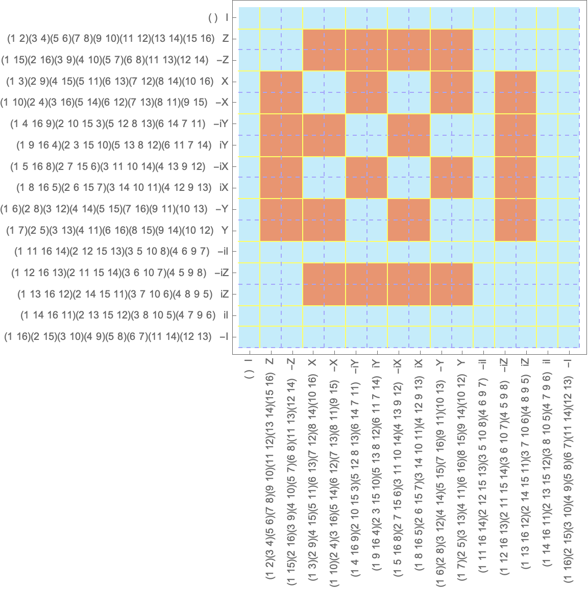
We can see that the center of the Pauli group is , each element there has its own conjugacy class, and then, interestingly each element has only one conjugate, which is -1 times the element itself.
The probability that two elements commute
The commutativity plot almost intuitively leads to this question: how dense can the blue squares be? In probabilistic terms, the proportion of the blue vs the full area is equivalent to the probability that two random elements commute from . Of course, we are interested in non-abelian groups, as abelian groups have a boring full-blue plot. In the case of , the plot becomes very large (6! x 6!), but we can see that it is very sparse (also has some cool structure in there):
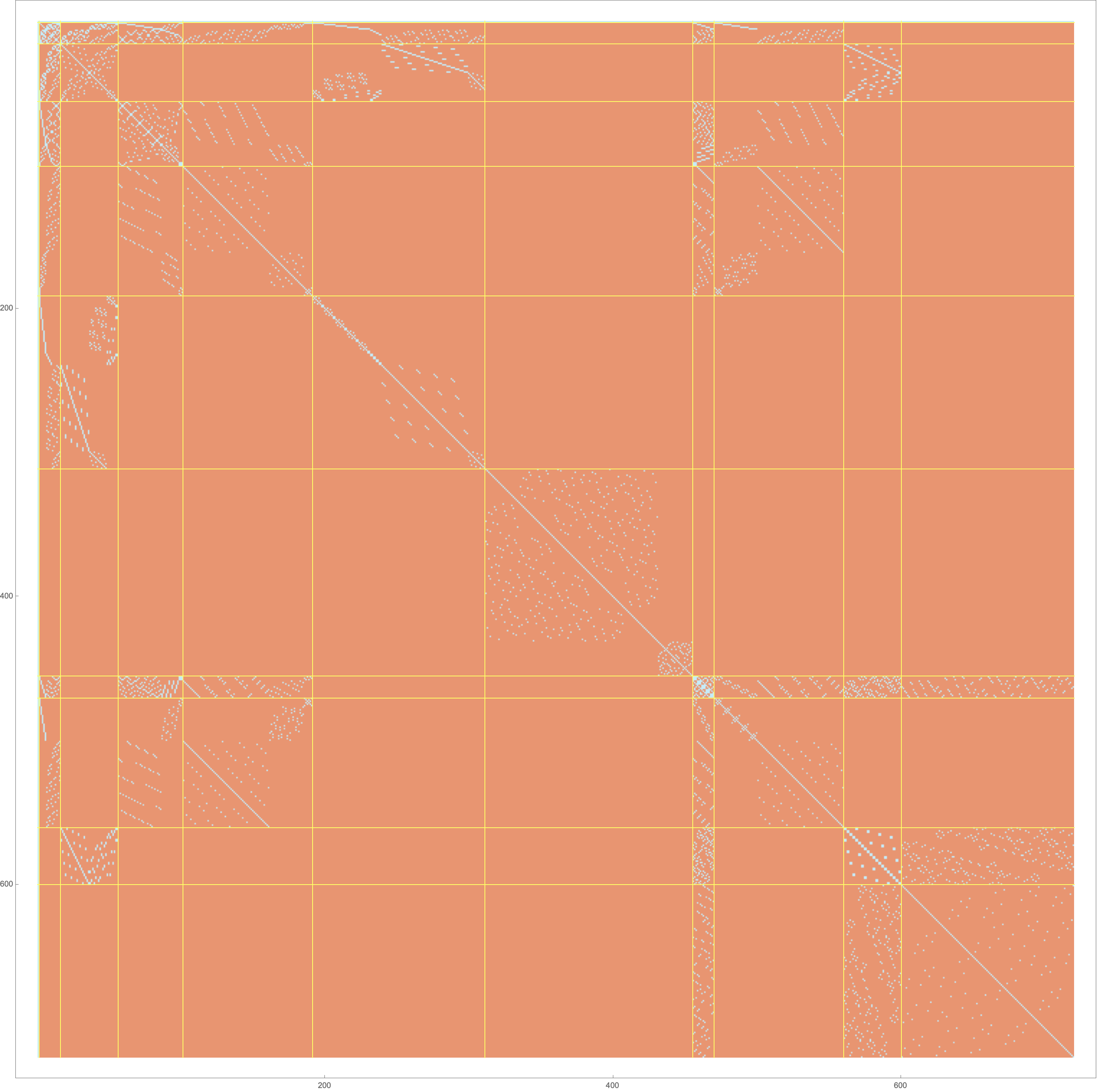
The Pauli group above and the quaternion group have much more blue in them. Let’s quantify this probability exactly.
CommutationProbability[group_] :=
 Count[Tuples[GroupElements[group], 2],
   x_ /;
    PermutationProduct[x[[1]], x[[2]]] ==
     PermutationProduct[x[[2]], x[[1]]]]/GroupOrder[group]^2
With the function above (again, very slow, brute force implementation, careful), we can see that our groups have the following probabilities of two of their elements to commute:
- abelian groups of course 100%
- Symmetric group of order 6: 11/720 - pretty low!
- Quaternion group, Dihedral group of order 4, and the Pauli group: 5/8
Can we go higher? It turns out that two random elements in a non-abelian group can’t have more than a 5/8 chance to commute!
The proof is relatively simple: given that the centralizer for any element in a non-abelian group is a proper subgroup, it can only be of order at most (due to Lagrange the subgroup’s order has to divide the group’s order). But, the same is true for the center of the group itself, is a subgroup of all the centralizers, and as such, it must be up to half the size of the centralizers, and as such, it must be that . We can see in the Pauli group that the center has 4 elements, out of the 16, we are hitting this limit.
Now, let’s use these bounds. We’ll simply add all the blue squares - that’s going to be all the orders of the centralizers of all the elements, and divide by all the squares, which is simply .
For elements in the center, the centralizer is the group itself (they commute with every element), so we can separate those out from the sum:
Let’s divide in with the order of :
And let’s use our bounds: and for all :
When I first saw this, my mind was blown - group theory seems like this area of infinite possibilities, but it seems like it contains a lot more structure than we’d think at first.
Conclusion
We demonstrated a simple tool to visualize commutation relationships within finite groups. It leverages the permutation representation of groups, which allows for a natural ordering that simplifies grouping conjugation classes together. We demonstrated proofs aided by this visual language for two theorems. I hope you enjoyed it, learned something from it!
Further things to explore and improve
This is probably just the tip of the iceberg. If I had an infinite amount of time I would explore a couple of ideas:
- Are these “game-of-life” type structures/patterns that show up in the plot of any interest? Can we derive anything from patterns formed on the plot from this particular ordering? Can other orderings result in different insights?
- What else can we visualize in this plot:
- Can we represent normalizers?
- Can we represent subgroup structure in the commutation plot?
- Improve the tool:
- Make the tool interactive
- create a Python/Javascript version of it, so it doesn’t depend on non-opensource software
If you find issues with the post, please open an issue or PR to fix it!
Acknowledgment
Big thank you to Prof. Nathan Carter for his comments on this blogpost and finding a bug in the original proof.
Comments
Comments are provided by giscus and Github Discussions. You will have to login with your Github account to comment.
- Dummit, D. S., & Foote, R. M. (2003). Abstract Algebra. Wiley. https://books.google.com/books?id=KIGbCgAAQBAJ